Robust Kernel

This tutorial demonstrates the use of robust kernels in the context of outlier rejection. For this particular tutorial, we will be using the ICP (Iterative Closest Point) registration algorithm as the target problem where we want to deal with outliers. Even so, the theory applies to any given optimization problem and not just for ICP. For the moment the robust kernels have been only implemented for the PointToPlane ICP.

The notation and some of the kernels implemented in Open3D has been inspired by the publication “Analysis of Robust Functions for Registration Algorithms” [Babin2019]

Note:

This tutorial and the original implementation of the robust kernels in Open3D was contributed by Ignacio Vizzo and Cyrill Stachniss from the University of Bonn.

Point-to-plane ICP using Robust Kernels

The standard point-to-plane ICP algorithm [ChenAndMedioni1992] minimizes this objective function:

\begin{equation} E(\mathbf{T}) = \sum_{(\mathbf{p},\mathbf{q})\in\mathcal{K}}\big((\mathbf{p} - \mathbf{T}\mathbf{q})\cdot\mathbf{n}_{\mathbf{p}}\big)^{2}, \end{equation}

where \(\mathbf{n}_{\mathbf{p}}\) is the normal of point \(\mathbf{p}\) and \(\mathcal{K}\) is the correspondence set between the target point cloud \(\mathbf{P}\), and source point cloud \(\mathbf{Q}\).

If we call \(r_i(\mathbf{T})\) is \(i^\mathrm{th}\) the residual, for a given pair of correspondences \((\mathbf{p},\mathbf{q})\in\mathcal{K}\) we can rewrite the objective function as.

\begin{equation} E(\mathbf{T}) = \sum_{(\mathbf{p},\mathbf{q})\in\mathcal{K}}\big((\mathbf{p} - \mathbf{T}\mathbf{q})\cdot\mathbf{n}_{\mathbf{p}}\big)^{2} = \sum_{i=1}^{N} \big({r_i(\mathbf{T})}\big)^2 \end{equation}

The optimization problem above can also be solved by using the iteratively reweighted least-squares (IRLS) approach, which solves a sequence of weighted least squares problems:

\begin{equation} E(\mathbf{T}) = \sum_{i=1}^{N} w_i \big({r_i(\mathbf{T})}\big)^2 \end{equation}

Outlier Rejection with Robust Kernels

The main idea of a robust loss is to downweight large residuals that are assumed to be caused from outliers such that their influence on the solution is reduced. This is achieved by optimizing \(E(\mathbf{T})\) as:

\begin{equation} E(\mathbf{T}) = \sum_{(\mathbf{p},\mathbf{q})\in\mathcal{K}}\rho\big((\mathbf{p} - \mathbf{T}\mathbf{q})\cdot\mathbf{n}_{\mathbf{p}}\big) = \sum_{i=1}^{N} \rho\big({r_i(\mathbf{T})}\big), \end{equation}

where \(\rho(r)\) is also called the robust loss or kernel.

We can see that exists a relation between the optimization formulation in IRLS and the one that uses the robust loss function. By setting the weight \(w_i= \frac{1}{r_i(\mathbf{T})}\rho'(r_i(\mathbf{T}))\), we can solve the robust loss optimization problem using the existing techniques for weighted least-squares. Therefore, we can minimize the objective function using Gauss-Newton and determine increments by iteratively solving:

\begin{align} \left(\mathbf{J}^\top \mathbf{W} \mathbf{J}\right)^{-1}\mathbf{J}^\top\mathbf{W}\vec{r}, \end{align}

where \(\mathbf{W} \in \mathbb{R}^{N\times N}\) is a diagonal matrix containing weights \(w_i\) for each residual \(r_i\)

How to use Robust Kernels in Open3D

icp, multi_scale_icp can be called with a parameter TransformationEstimationPointToPlane(loss) or TransformationEstimationForColoredICP(loss). Where loss is a given loss function(also called robust kernel).

Internally, TransormationEstimationPointToPlane(loss) implements a function to compute the weighted residuals and Jacobian matrices of the point-to-plane ICP objective according to the provided robust kernel.

Vanilla ICP vs Robust ICP

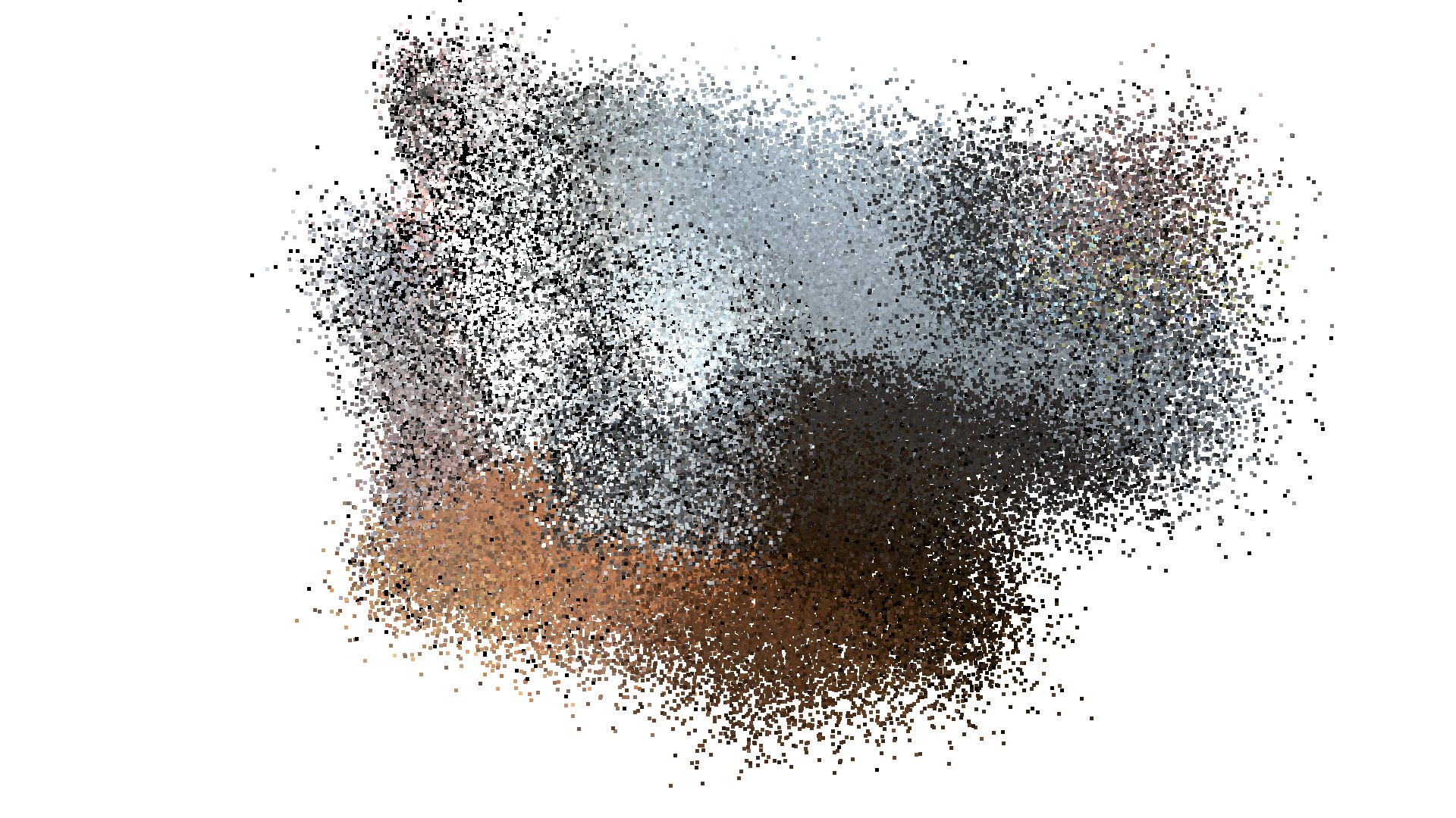
To better show the advantages of using robust kernels in the registration, we add some artificially generated gaussian noise to the source point cloud.

# Overriding visualization function, according to best camera view for colored-icp sample data.
def draw_registration_result(source, target, transformation):
    source_temp = source.clone()
    target_temp = target.clone()

    source_temp.transform(transformation)

    # This is patched version for tutorial rendering.
    # Use `draw` function for you application.
    o3d.visualization.draw_geometries(
        [source_temp.to_legacy(),
         target_temp.to_legacy()],
        zoom=0.4459,
        front=[0.9288, -0.2951, -0.2242],
        lookat=[1.6784, 2.0612, 1.4451],
        up=[-0.3402, -0.9189, -0.1996])

demo_icp_pcds = o3d.data.DemoICPPointClouds()
source = o3d.t.io.read_point_cloud(demo_icp_pcds.paths[0])
target = o3d.t.io.read_point_cloud(demo_icp_pcds.paths[1])

def apply_noise(pcd, mu, sigma):
    device = pcd.point["positions"].device
    noisy_pcd = pcd.cpu().clone()
    noisy_pcd.point["positions"] += o3d.core.Tensor(
        np.random.normal(mu, sigma, size=noisy_pcd.point["positions"].shape),
        noisy_pcd.point["positions"].dtype)
    return noisy_pcd


mu, sigma = 0, 0.1  # mean and standard deviation
source_noisy = apply_noise(source, mu, sigma)

print("Source PointCloud + noise:")
o3d.visualization.draw_geometries([source_noisy.to_legacy()],
                                  zoom=0.4459,
                                  front=[0.353, -0.469, -0.809],
                                  lookat=[2.343, 2.217, 1.809],
                                  up=[-0.097, -0.879, 0.467])

Source PointCloud + noise:

Vanilla ICP

We inspect how the results will look if we use the exact same parameters that were used in the above examples of ICP.

# Initial alignment or source to target transform.
init_source_to_target = np.asarray([[0.862, 0.011, -0.507, 0.5],
                                    [-0.139, 0.967, -0.215, 0.7],
                                    [0.487, 0.255, 0.835, -1.4],
                                    [0.0, 0.0, 0.0, 1.0]])

criteria = treg.ICPConvergenceCriteria(relative_fitness=0.000001,
                                       relative_rmse=0.000001,
                                       max_iteration=50)

estimation = treg.TransformationEstimationPointToPlane()

max_correspondence_distance = 0.02

print("Vanilla point-to-plane ICP, max_correspondence_distance={}:".format(
    max_correspondence_distance))
s = time.time()

reg_point_to_plane = treg.icp(source_noisy, target, max_correspondence_distance,
                              init_source_to_target, estimation)

icp_time = time.time() - s

print("Time taken by Point-To-Plane ICP: ", icp_time)
print("Fitness: ", reg_point_to_plane.fitness)
print("Inlier RMSE: ", reg_point_to_plane.inlier_rmse)

draw_registration_result(source, target, reg_point_to_plane.transformation)

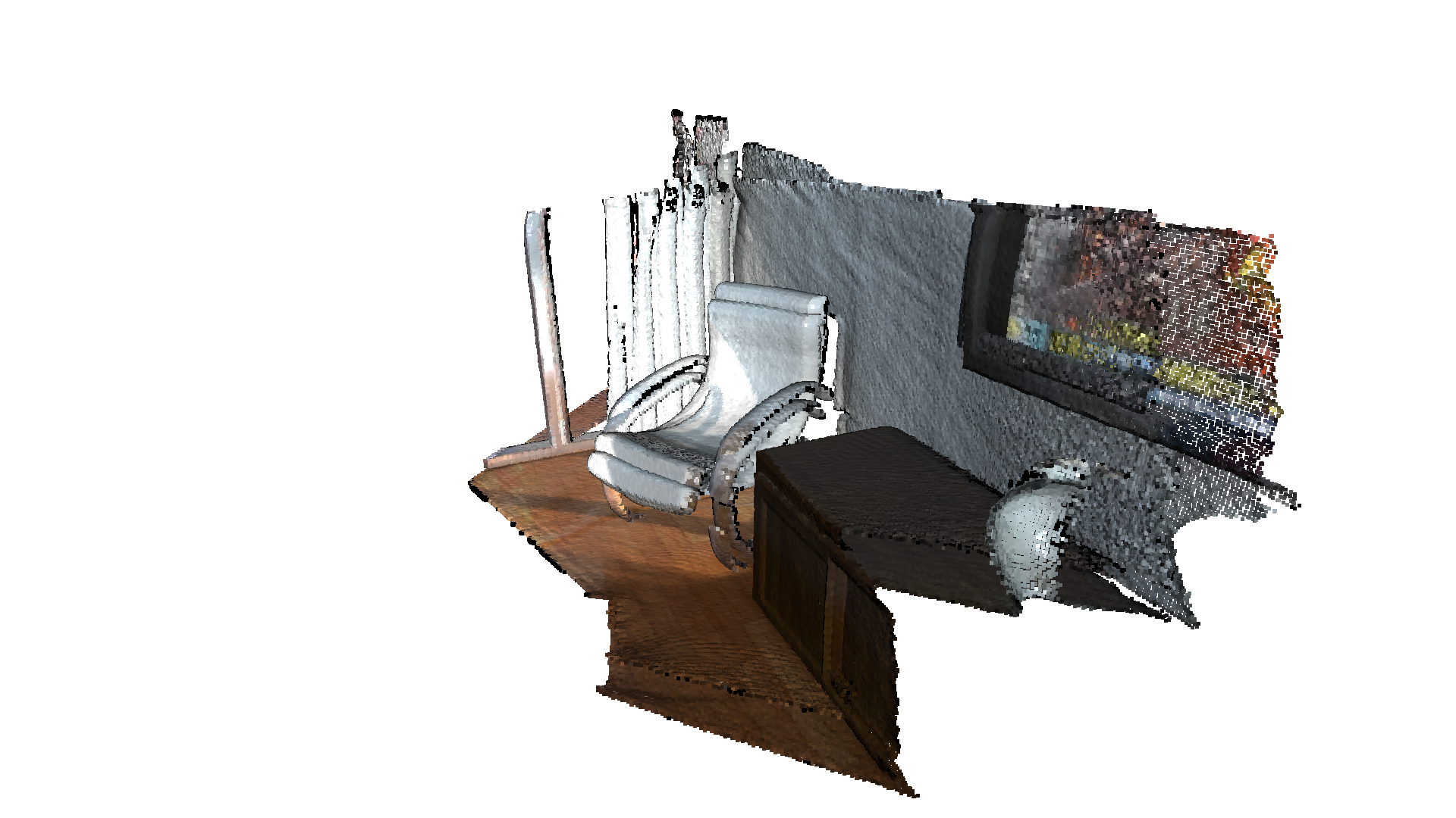
Vanilla point-to-plane ICP, max_correspondence_distance=0.02:
Time taken by Point-To-Plane ICP:  0.990375280380249
Fitness:  0.09650212487741092
Inlier RMSE:  0.011948867219549538

Tuning Vanilla ICP

Given the fact that we are now dealing with gaussian noise, we might try to increase the threshold to search for nearest neighbors with the aim of improving the registration result.

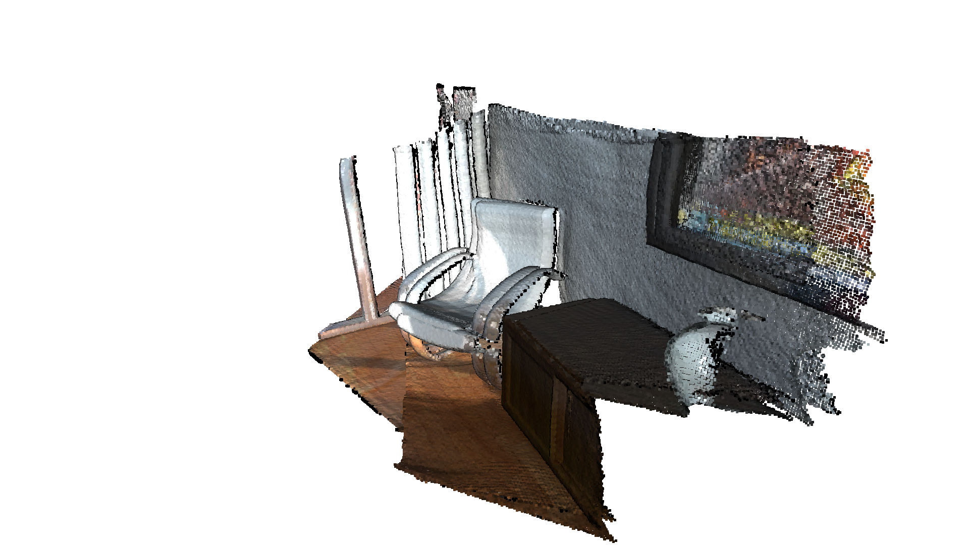
We can see that under these conditions and without a robust kernel, the traditional ICP has no chance to deal with outliers.

estimation = treg.TransformationEstimationPointToPlane()

max_correspondence_distance = 0.5

voxel_size = 0.02

print("Vanilla point-to-plane ICP, max_correspondence_distance={}:".format(
    max_correspondence_distance))

s = time.time()

reg_point_to_plane = treg.icp(source, target, max_correspondence_distance,
                              init_source_to_target, estimation, criteria,
                              voxel_size)

icp_time = time.time() - s

print("Time taken by Point-To-Plane ICP: ", icp_time)
print("Fitness: ", reg_point_to_plane.fitness)
print("Inlier RMSE: ", reg_point_to_plane.inlier_rmse)

draw_registration_result(source, target, reg_point_to_plane.transformation)

Vanilla point-to-plane ICP, max_correspondence_distance=0.5:
Time taken by Point-To-Plane ICP:  17.679412841796875
Fitness:  0.8304424518594737
Inlier RMSE:  0.13779966614181124

Robust ICP

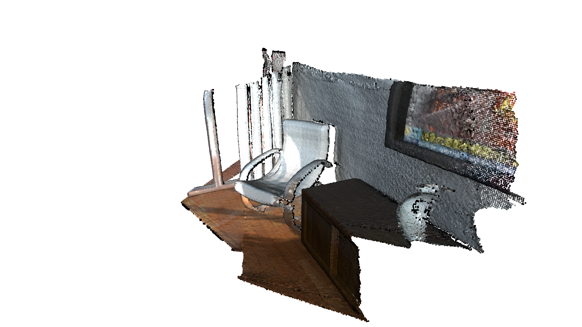
Using the same max_correspondence_distance=0.5 and a robust kernel, we can properly register the two point clouds:

mu, sigma = 0, 0.1  # mean and standard deviation
estimation = treg.TransformationEstimationPointToPlane(
    treg.robust_kernel.RobustKernel(
        treg.robust_kernel.RobustKernelMethod.TukeyLoss, sigma))

print("Vanilla point-to-plane ICP, max_correspondence_distance={}:".format(
    max_correspondence_distance))

s = time.time()

reg_point_to_plane = treg.icp(source, target, max_correspondence_distance,
                              init_source_to_target, estimation, criteria,
                              voxel_size)

icp_time = time.time() - s
print("Time taken by Point-To-Plane ICP: ", icp_time)
print("Fitness: ", reg_point_to_plane.fitness)
print("Inlier RMSE: ", reg_point_to_plane.inlier_rmse)

draw_registration_result(source, target, reg_point_to_plane.transformation)

Vanilla point-to-plane ICP, max_correspondence_distance=0.5:
Time taken by Point-To-Plane ICP:  10.51712417602539
Fitness:  0.810708510951051
Inlier RMSE:  0.13371120372728632

Registration estimation method supports Robust Kernels:

robust_kernel = o3d.t.pipelines.registration.robust_kernel.RobustKernel(method, scale, shape)

Method options:

• robust_kernel.RobustKernelMethod.L2Loss

• robust_kernel.RobustKernelMethod.L1Loss

• robust_kernel.RobustKernelMethod.HuberLoss

• robust_kernel.RobustKernelMethod.CauchyLoss

• robust_kernel.RobustKernelMethod.GMLoss

• robust_kernel.RobustKernelMethod.TukeyLoss

• robust_kernel.RobustKernelMethod.GeneralizedLoss

Note:

For this example we use the TukeyLoss. For the parameter k we set it to match the std deviation of the noise model \(k = \sigma\). The parameter k used in the Robust Kernels it’s usually pick to match the standard deviation of the noise model of the input data. In this sense, k, is the discriminator between inlier/outlier. Although this is not always trivial to define in real world data, for synthetic one, it’s easy to fix in order to illustrate the benefits of the robust kernels.

---