[1]:
import open3d as o3d
import open3d.core as o3c
import numpy as np
import matplotlib.pyplot as plt
import copy
import os
import sys

# Only needed for tutorial, monkey patches visualization
sys.path.append("..")
import open3d_tutorial as o3dtut
# Change to True if you want to interact with the visualization windows
o3dtut.interactive = not "CI" in os.environ
Using external Open3D-ML in /home/runner/work/Open3D/Open3D/Open3D-ML
PointCloud#
This tutorial demonstrates basic usage of a point cloud.
PointCloud creation#
The first part of the tutorial shows how to construct a point cloud.
[2]:
# Create a empty point cloud on CPU.
pcd = o3d.t.geometry.PointCloud()
print(pcd, "\n")

# To create a point cloud on CUDA, specify the device.
# pcd = o3d.t.geometry.PointCloud(o3c.Device("cuda:0"))

# Create a point cloud from open3d tensor with dtype of float32.
pcd = o3d.t.geometry.PointCloud(o3c.Tensor([[0, 0, 0], [1, 1, 1]], o3c.float32))
print(pcd, "\n")

# Create a point cloud from open3d tensor with dtype of float64.
pcd = o3d.t.geometry.PointCloud(o3c.Tensor([[0, 0, 0], [1, 1, 1]], o3c.float64))
print(pcd, "\n")

# Create a point cloud from numpy array. The array will be copied.
pcd = o3d.t.geometry.PointCloud(
    np.array([[0, 0, 0], [1, 1, 1]], dtype=np.float32))
print(pcd, "\n")

# Create a point cloud from python list.
pcd = o3d.t.geometry.PointCloud([[0., 0., 0.], [1., 1., 1.]])
print(pcd, "\n")

# Error creation. The point cloud must have shape of (N, 3).
try:
    pcd = o3d.t.geometry.PointCloud(o3c.Tensor([0, 0, 0, 0], o3c.float32))
except:
    print(f"Error creation. The point cloud must have shape of (N, 3).")
PointCloud on CPU:0 [0 points].
Attributes: None.

PointCloud on CPU:0 [2 points (Float32)].
Attributes: None.

PointCloud on CPU:0 [2 points (Float64)].
Attributes: None.

PointCloud on CPU:0 [2 points (Float32)].
Attributes: None.

PointCloud on CPU:0 [2 points (Float64)].
Attributes: None.

Error creation. The point cloud must have shape of (N, 3).
The PointCloud can be created on both CPU and GPU, and with different data types. The device of the point cloud will be the same as the device of the input tensor.
Besides, PointCloud can be also created by python dict with multiple attributes.
[3]:
map_to_tensors = {}

# - The "positions" attribute must be specified.
# - Common attributes include "colors" and "normals".
# - You may also use custom attributes, such as "labels".
# - The value of an attribute could be of any shape and dtype. Its correctness
#   will only be checked when the attribute is used by some algorithms.
map_to_tensors["positions"] = o3c.Tensor([[0, 0, 0], [1, 1, 1]], o3c.float32)
map_to_tensors["normals"] = o3c.Tensor([[0, 0, 1], [0, 0, 1]], o3c.float32)
map_to_tensors["labels"] = o3c.Tensor([0, 1], o3c.int64)

pcd = o3d.t.geometry.PointCloud(map_to_tensors)
print(pcd)
PointCloud on CPU:0 [2 points (Float32)].
Attributes: normals (dtype = Float32, shape = {2, 3}), labels (dtype = Int64, shape = {2}).
Point cloud attributes setter and getter#
[4]:
pcd = o3d.t.geometry.PointCloud(o3c.Tensor([[0, 0, 0], [1, 1, 1]], o3c.float32))
# Set attributes.
pcd.point.normals = o3c.Tensor([[0, 0, 1], [0, 0, 1]], o3c.float32)
pcd.point.colors = o3c.Tensor([[1, 0, 0], [0, 1, 0]], o3c.float32)
pcd.point.labels = o3c.Tensor([0, 1], o3c.int64)
print(pcd, "\n")

# Set by numpy array or python list.
pcd.point.normals = np.array([[0, 0, 1], [0, 0, 1]], dtype=np.float32)
pcd.point.intensity = [0.4, 0.4]
print(pcd, "\n")

# Get attributes.
posisions = pcd.point.positions
print("posisions: ")
print(posisions, "\n")
labels = pcd.point.labels
print("labels: ")
print(labels, "")
PointCloud on CPU:0 [2 points (Float32)].
Attributes: labels (dtype = Int64, shape = {2}), colors (dtype = Float32, shape = {2, 3}), normals (dtype = Float32, shape = {2, 3}).

PointCloud on CPU:0 [2 points (Float32)].
Attributes: labels (dtype = Int64, shape = {2}), colors (dtype = Float32, shape = {2, 3}), normals (dtype = Float32, shape = {2, 3}), intensity (dtype = Float64, shape = {2}).

posisions:
[[0 0 0],
 [1 1 1]]
Tensor[shape={2, 3}, stride={3, 1}, Float32, CPU:0, 0x5636eb68b8d0]

labels:
[0 1]
Tensor[shape={2}, stride={1}, Int64, CPU:0, 0x5636ebcd36c0]
Conversion between tensor and legacy point cloud#
PointCloud can be converted to/from legacy open3d.geometry.PointCloud.
[5]:
legacy_pcd = pcd.to_legacy()
print(legacy_pcd, "\n")

tensor_pcd = o3d.t.geometry.PointCloud.from_legacy(legacy_pcd)
print(tensor_pcd, "\n")

# Convert from legacy point cloud with data type of float64.
tensor_pcd_f64 = o3d.t.geometry.PointCloud.from_legacy(legacy_pcd, o3c.float64)
print(tensor_pcd_f64, "\n")
PointCloud with 2 points.

PointCloud on CPU:0 [2 points (Float32)].
Attributes: normals (dtype = Float32, shape = {2, 3}), colors (dtype = Float32, shape = {2, 3}).

PointCloud on CPU:0 [2 points (Float64)].
Attributes: normals (dtype = Float64, shape = {2, 3}), colors (dtype = Float64, shape = {2, 3}).
Visualize point cloud#
[6]:
print("Load a ply point cloud, print it, and render it")
ply_point_cloud = o3d.data.PLYPointCloud()
pcd = o3d.t.io.read_point_cloud(ply_point_cloud.path)
print(pcd)
o3d.visualization.draw_geometries([pcd.to_legacy()],
                                  zoom=0.3412,
                                  front=[0.4257, -0.2125, -0.8795],
                                  lookat=[2.6172, 2.0475, 1.532],
                                  up=[-0.0694, -0.9768, 0.2024])
Load a ply point cloud, print it, and render it
[Open3D INFO] Downloading https://github.com/isl-org/open3d_downloads/releases/download/20220201-data/fragment.ply
[Open3D INFO] Downloaded to /home/runner/open3d_data/download/PLYPointCloud/fragment.ply
PointCloud on CPU:0 [196133 points (Float32)].
Attributes: curvature (dtype = Float32, shape = {196133, 1}), normals (dtype = Float32, shape = {196133, 3}), colors (dtype = UInt8, shape = {196133, 3}).
[Open3D WARNING] GLFW Error: Failed to detect any supported platform
[Open3D WARNING] GLFW initialized for headless rendering.

read_point_cloud reads a point cloud from a file. It tries to decode the file based on the extension name. For a list of supported file types, refer to File IO.
draw_geometries visualizes the point cloud. Use a mouse/trackpad to see the geometry from different view points.
It looks like a dense surface, but it is actually a point cloud rendered as surfels. The GUI supports various keyboard functions. For instance, the - key reduces the size of the points (surfels).
Note:
Press the H key to print out a complete list of keyboard instructions for the GUI. For more information of the visualization GUI, refer to Visualization and Customized visualization.
Note:
On macOS, the GUI window may not receive keyboard events. In this case, try to launch Python with pythonw instead of python.
Downsampling#
This section provides several downsamle methods of a point cloud. ### Voxel downsampling Voxel downsampling uses a regular voxel grid to create a uniformly downsampled point cloud from an input point cloud. It is often used as a pre-processing step for many point cloud processing tasks. The algorithm operates in two steps:
Points are bucketed into voxels.
Each occupied voxel generates exactly one point by averaging all points inside.
Note:
Currently, the method returns the voxel coordinates of the point cloud.
[7]:
print("Downsample the point cloud with a voxel of 0.03")
downpcd = pcd.voxel_down_sample(voxel_size=0.03)
o3d.visualization.draw_geometries([downpcd.to_legacy()],
                                  zoom=0.3412,
                                  front=[0.4257, -0.2125, -0.8795],
                                  lookat=[2.6172, 2.0475, 1.532],
                                  up=[-0.0694, -0.9768, 0.2024])
Downsample the point cloud with a voxel of 0.03
[Open3D WARNING] GLFW initialized for headless rendering.

Farthest point downsampling#
Farthest point sampling samples the point cloud by selecting the farthest point from the current selected point iteratively. It is used to sample the point cloud to a fixed number of points which holds the maximum geometrical information of the original point cloud.
[8]:
print("Downsample the point cloud by selecting 5000 farthest points.")
downpcd_farthest = pcd.farthest_point_down_sample(5000)
o3d.visualization.draw_geometries([downpcd_farthest.to_legacy()],
                                  zoom=0.3412,
                                  front=[0.4257, -0.2125, -0.8795],
                                  lookat=[2.6172, 2.0475, 1.532],
                                  up=[-0.0694, -0.9768, 0.2024])
Downsample the point cloud by selecting 5000 farthest points.
[Open3D WARNING] GLFW initialized for headless rendering.

Open3D also provides uniform_down_sample and random_down_sample for point cloud downsampling.
Vertex normal estimation#
Another basic operation for point cloud is normal estimation. Press N to see point normals. The keys - and + can be used to control the length of the normal.
[9]:
print("Recompute the normal of the downsampled point cloud using hybrid nearest neighbor search with 30 max_nn and radius of 0.1m.")
downpcd.estimate_normals(max_nn=30, radius=0.1)
o3d.visualization.draw_geometries([downpcd.to_legacy()],
                                  zoom=0.3412,
                                  front=[0.4257, -0.2125, -0.8795],
                                  lookat=[2.6172, 2.0475, 1.532],
                                  up=[-0.0694, -0.9768, 0.2024],
                                  point_show_normal=True)
Recompute the normal of the downsampled point cloud using hybrid nearest neighbor search with 30 max_nn and radius of 0.1m.
[Open3D WARNING] GLFW initialized for headless rendering.

estimate_normals computes the normal for every point. The function finds adjacent points and calculates the principal axis of the adjacent points using covariance analysis.
The two key arguments radius = 0.1 and max_nn = 30 specifies search radius and maximum nearest neighbor. It has 10cm of search radius, and only considers up to 30 neighbors to save computation time. If only max_nn or radius is specified (downpcd.estimate_normals(30, None) or downpcd.estimate_normals(None, 0.01)), the function will use knn or radius search respectively.
Note: It is always recommended to specify both radius and max_nn, especially if the point cloud is on CUDA device.
Note: The covariance analysis algorithm produces two opposite directions as normal candidates. Without knowing the global structure of the geometry, both can be correct. This is known as the normal orientation problem. Open3D tries to orient the normal to align with the original normal if it exists. Otherwise, Open3D does a random guess. Further orientation functions such as orient_normals_to_align_with_direction and orient_normals_towards_camera_location need to be called if the
orientation is a concern.
Access estimated normals#
The estimated normals can be access and converted to numpy array.
[10]:
normals = downpcd.point.normals
print("Print first 5 normals of the downsampled point cloud.")
print(normals[:5], "\n")
print("Convert normals tensor into numpy array.")
normals_np = normals.numpy()
print(normals_np[:5])
Print first 5 normals of the downsampled point cloud.
[[-0.48448014 0.16192137 -0.85968626],
 [-0.4547148 0.17396295 -0.8734824],
 [-0.42535082 0.12960345 -0.8957007],
 [-0.4281835 0.124074414 -0.89513385],
 [-0.51735884 0.2142542 -0.8285136]]
Tensor[shape={5, 3}, stride={3, 1}, Float32, CPU:0, 0x5636edc2aa90]

Convert normals tensor into numpy array.
[[-0.48448014  0.16192137 -0.85968626]
 [-0.4547148   0.17396295 -0.8734824 ]
 [-0.42535082  0.12960345 -0.8957007 ]
 [-0.4281835   0.12407441 -0.89513385]
 [-0.51735884  0.2142542  -0.8285136 ]]
Crop point cloud#
[11]:
print("Load a polygon volume and use it to crop the original point cloud")
demo_crop_data = o3d.data.DemoCropPointCloud()
pcd = o3d.t.io.read_point_cloud(demo_crop_data.point_cloud_path)
vol = o3d.visualization.read_selection_polygon_volume(demo_crop_data.cropped_json_path)
chair = vol.crop_point_cloud(pcd.to_legacy())
o3d.visualization.draw_geometries([chair],
                                  zoom=0.7,
                                  front=[0.5439, -0.2333, -0.8060],
                                  lookat=[2.4615, 2.1331, 1.338],
                                  up=[-0.1781, -0.9708, 0.1608])
Load a polygon volume and use it to crop the original point cloud
[Open3D INFO] Downloading https://github.com/isl-org/open3d_downloads/releases/download/20220201-data/DemoCropPointCloud.zip
[Open3D INFO] Downloaded to /home/runner/open3d_data/download/DemoCropPointCloud/DemoCropPointCloud.zip
[Open3D INFO] Created directory /home/runner/open3d_data/extract/DemoCropPointCloud.
[Open3D INFO] Extracting /home/runner/open3d_data/download/DemoCropPointCloud/DemoCropPointCloud.zip.
[Open3D INFO] Extracted to /home/runner/open3d_data/extract/DemoCropPointCloud.
[Open3D WARNING] GLFW initialized for headless rendering.

read_selection_polygon_volume reads a json file that specifies polygon selection area. vol.crop_point_cloud(pcd) filters out points. Only the chair remains.
We can also get the cropped indices of the point cloud using crop_in_polygon.
[12]:
indices = vol.crop_in_polygon(pcd.to_legacy())
print(f"Cropped indices length: {len(indices)}")
Cropped indices length: 31337
Paint point cloud#
[13]:
print("Paint point cloud.")
pcd.paint_uniform_color([1, 0.706, 0])
o3d.visualization.draw_geometries([pcd.to_legacy()],
                                  zoom=0.7,
                                  front=[0.5439, -0.2333, -0.8060],
                                  lookat=[2.4615, 2.1331, 1.338],
                                  up=[-0.1781, -0.9708, 0.1608])
Paint point cloud.
[Open3D WARNING] GLFW initialized for headless rendering.

paint_uniform_color paints all the points to a uniform color. The color is in RGB space, [0, 1] range.
Bounding volumes#
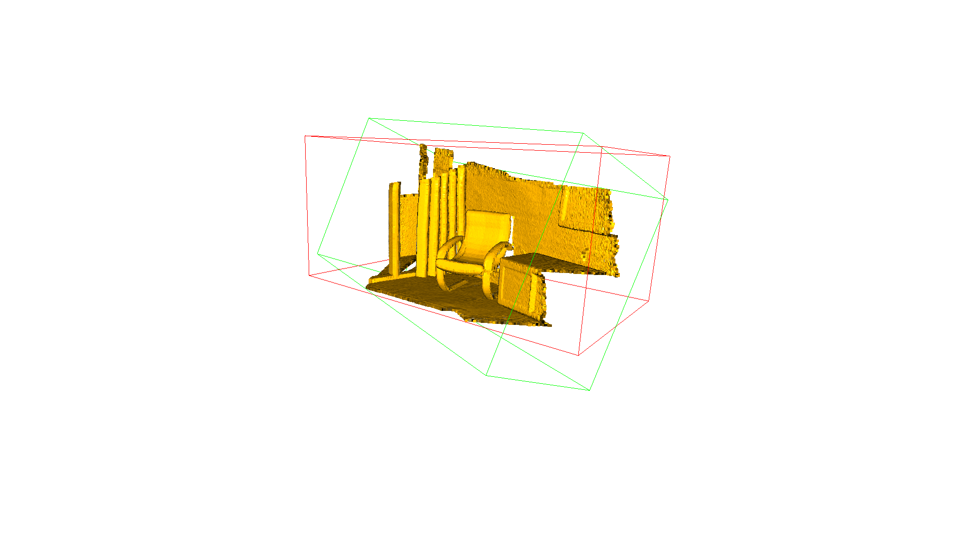
The PointCloud geometry type has bounding volumes as all other geometry types in Open3D. Currently, Open3D implements an AxisAlignedBoundingBox and an OrientedBoundingBox that can also be used to crop the geometry.
[14]:
aabb = pcd.get_axis_aligned_bounding_box()
aabb.set_color(o3c.Tensor([1, 0, 0], o3c.float32))
obb = pcd.get_oriented_bounding_box()
obb.set_color(o3c.Tensor([0, 1, 0], o3c.float32))
o3d.visualization.draw_geometries(
    [pcd.to_legacy(), aabb.to_legacy(),
     obb.to_legacy()],
    zoom=0.7,
    front=[0.5439, -0.2333, -0.8060],
    lookat=[2.4615, 2.1331, 1.338],
    up=[-0.1781, -0.9708, 0.1608])
[Open3D WARNING] GLFW initialized for headless rendering.
Point cloud outlier removal#
When collecting data from scanning devices, the resulting point cloud tends to contain noise and artifacts that one would like to remove. This demo below addresses the outlier removal features of Open3D.
Prepare input data#
A point cloud is loaded and downsampled using voxel_downsample.
[15]:
print("Load a ply point cloud, print it, and render it")
sample_pcd_data = o3d.data.PCDPointCloud()
pcd = o3d.t.io.read_point_cloud(sample_pcd_data.path)
o3d.visualization.draw_geometries([pcd.to_legacy()],
                                  zoom=0.3412,
                                  front=[0.4257, -0.2125, -0.8795],
                                  lookat=[2.6172, 2.0475, 1.532],
                                  up=[-0.0694, -0.9768, 0.2024])

print("Downsample the point cloud with a voxel of 0.02")
voxel_down_pcd = pcd.voxel_down_sample(voxel_size=0.02)
o3d.visualization.draw_geometries([voxel_down_pcd.to_legacy()],
                                  zoom=0.3412,
                                  front=[0.4257, -0.2125, -0.8795],
                                  lookat=[2.6172, 2.0475, 1.532],
                                  up=[-0.0694, -0.9768, 0.2024])
Load a ply point cloud, print it, and render it
[Open3D INFO] Downloading https://github.com/isl-org/open3d_downloads/releases/download/20220201-data/fragment.pcd
[Open3D INFO] Downloaded to /home/runner/open3d_data/download/PCDPointCloud/fragment.pcd
[Open3D WARNING] GLFW initialized for headless rendering.

Downsample the point cloud with a voxel of 0.02
[Open3D WARNING] GLFW initialized for headless rendering.

Alternatively, use uniform_down_sample to downsample the point cloud by collecting every n-th points.
[16]:
print("Every 5th points are selected")
uni_down_pcd = pcd.uniform_down_sample(every_k_points=5)
o3d.visualization.draw_geometries([uni_down_pcd.to_legacy()],
                                  zoom=0.3412,
                                  front=[0.4257, -0.2125, -0.8795],
                                  lookat=[2.6172, 2.0475, 1.532],
                                  up=[-0.0694, -0.9768, 0.2024])
Every 5th points are selected
[Open3D WARNING] GLFW initialized for headless rendering.

Select down sample#
The following helper function uses select_by_mask, which takes a binary mask to output only the selected points. The selected points and the non-selected points are visualized.
[17]:
def display_inlier_outlier(cloud : o3d.t.geometry.PointCloud, mask : o3c.Tensor):
    inlier_cloud = cloud.select_by_mask(mask)
    outlier_cloud = cloud.select_by_mask(mask, invert=True)

    print("Showing outliers (red) and inliers (gray): ")
    outlier_cloud = outlier_cloud.paint_uniform_color([1.0, 0, 0])
    inlier_cloud.paint_uniform_color([0.8, 0.8, 0.8])
    inlier_cloud = o3d.visualization.draw_geometries([inlier_cloud.to_legacy(), outlier_cloud.to_legacy()],
                                      zoom=0.3412,
                                      front=[0.4257, -0.2125, -0.8795],
                                      lookat=[2.6172, 2.0475, 1.532],
                                      up=[-0.0694, -0.9768, 0.2024])
Statistical outlier removal#
statistical_outlier_removal removes points that are further away from their neighbors compared to the average for the point cloud. It takes two input parameters:
nb_neighbors, which specifies how many neighbors are taken into account in order to calculate the average distance for a given point.std_ratio, which allows setting the threshold level based on the standard deviation of the average distances across the point cloud. The lower this number the more aggressive the filter will be.
[18]:
print("Statistical oulier removal")
cl, ind = voxel_down_pcd.remove_statistical_outliers(nb_neighbors=20,
                                                     std_ratio=2.0)
display_inlier_outlier(voxel_down_pcd, ind)
Statistical oulier removal
Showing outliers (red) and inliers (gray):
[Open3D WARNING] GLFW initialized for headless rendering.

Radius outlier removal#
radius_outlier_removal removes points that have few neighbors in a given sphere around them. Two parameters can be used to tune the filter to your data:
nb_points, which lets you pick the minimum amount of points that the sphere should contain.radius, which defines the radius of the sphere that will be used for counting the neighbors.
[19]:
print("Radius oulier removal")
cl, ind = voxel_down_pcd.remove_radius_outliers(nb_points=16, search_radius=0.05)
display_inlier_outlier(voxel_down_pcd, ind)
Radius oulier removal
Showing outliers (red) and inliers (gray):
[Open3D WARNING] GLFW initialized for headless rendering.

Convex hull#
The convex hull of a point cloud is the smallest convex set that contains all points. Open3D contains the method compute_convex_hull that computes the convex hull of a point cloud. The implementation is based on Qhull.
In the example code below we compute the convex hull that is returned as a triangle mesh. Then, we visualize the convex hull as a red LineSet.
[20]:
bunny = o3d.data.BunnyMesh()
pcd = o3d.t.io.read_point_cloud(bunny.path)

hull = pcd.compute_convex_hull()
hull_ls = o3d.geometry.LineSet.create_from_triangle_mesh(hull.to_legacy())
hull_ls.paint_uniform_color((1, 0, 0))
o3d.visualization.draw_geometries([pcd.to_legacy(), hull_ls])
[Open3D INFO] Downloading https://github.com/isl-org/open3d_downloads/releases/download/20220201-data/BunnyMesh.ply
[Open3D INFO] Downloaded to /home/runner/open3d_data/download/BunnyMesh/BunnyMesh.ply
[Open3D WARNING] GLFW initialized for headless rendering.
DBSCAN clustering#
Given a point cloud from e.g. a depth sensor we want to group local point cloud clusters together. For this purpose, we can use clustering algorithms. Open3D implements DBSCAN [Ester1996] that is a density based clustering algorithm. The algorithm is implemented in cluster_dbscan and requires two parameters: eps defines the distance to neighbors in a cluster and min_points defines the minimum number of points required to form a cluster. The function
returns labels, where the label -1 indicates noise.
[21]:
ply_point_cloud = o3d.data.PLYPointCloud()
pcd = o3d.t.io.read_point_cloud(ply_point_cloud.path)

with o3d.utility.VerbosityContextManager(
        o3d.utility.VerbosityLevel.Debug) as cm:
    labels = pcd.cluster_dbscan(eps=0.02, min_points=10, print_progress=True)

max_label = labels.max().item()
print(f"point cloud has {max_label + 1} clusters")
colors = plt.get_cmap("tab20")(
        labels.numpy() / (max_label if max_label > 0 else 1))
colors = o3c.Tensor(colors[:, :3], o3c.float32)
colors[labels < 0] = 0
pcd.point.colors = colors
o3d.visualization.draw_geometries([pcd.to_legacy()],
                                  zoom=0.455,
                                  front=[-0.4999, -0.1659, -0.8499],
                                  lookat=[2.1813, 2.0619, 2.0999],
                                  up=[0.1204, -0.9852, 0.1215])
[Open3D DEBUG] Precompute neighbors.
[Open3D DEBUG] Done Precompute neighbors.
[Open3D DEBUG] Compute Clusters
Precompute neighbors.[========================================] 100%
Clustering[Open3D DEBUG] Done Compute Clusters: 10
point cloud has 10 clusters
[Open3D WARNING] GLFW initialized for headless rendering.

Note:
This algorithm precomputes all neighbors in the epsilon radius for all points. This can require a lot of memory if the chosen epsilon is too large.
Plane segmentation#
Open3D also supports segmententation of geometric primitives from point clouds using RANSAC. To find the plane with the largest support in the point cloud, we can use segment_plane. The method has four arguments: distance_threshold defines the maximum distance a point can have to an estimated plane to be considered an inlier, ransac_n defines the number of points that are randomly sampled to estimate a plane, num_iterations defines how often a random plane is sampled and
verified, and probability defined the expected probability of finding the optimal plane. The function then returns the plane as
[22]:
sample_pcd_data = o3d.data.PCDPointCloud()
pcd = o3d.t.io.read_point_cloud(sample_pcd_data.path)
plane_model, inliers = pcd.segment_plane(distance_threshold=0.01,
                                            ransac_n=3,
                                            num_iterations=1000,
                                            probability=0.9999)
[a, b, c, d] = plane_model.numpy().tolist()
print(f"Plane equation: {a:.2f}x + {b:.2f}y + {c:.2f}z + {d:.2f} = 0")

inlier_cloud = pcd.select_by_index(inliers)
inlier_cloud = inlier_cloud.paint_uniform_color([1.0, 0, 0])
outlier_cloud = pcd.select_by_index(inliers, invert=True)
o3d.visualization.draw_geometries([inlier_cloud.to_legacy(), outlier_cloud.to_legacy()],
                                  zoom=0.8,
                                  front=[-0.4999, -0.1659, -0.8499],
                                  lookat=[2.1813, 2.0619, 2.0999],
                                  up=[0.1204, -0.9852, 0.1215])
Plane equation: -0.06x + -0.10y + 0.99z + -1.06 = 0
[Open3D WARNING] GLFW initialized for headless rendering.

To achieve the stable results with specific random seed, you can set probability to 1.0, which will force the executed iteration equal to num_iterations. (Since 0.16.0, the segment_plane function is parallel, and the iteration will be updated by the equation: iter = log(1 - probability) / log(1 - fitness ^ ransac_n), where fitness is the ratio of inliers number and total number of points)
[23]:
o3d.utility.random.seed(0)

plane_model, inliers = pcd.segment_plane(distance_threshold=0.01,
                                            ransac_n=3,
                                            num_iterations=1000,
                                            probability=1.0)
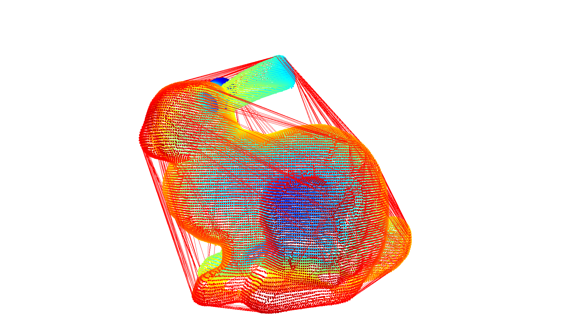
Hidden point removal#
Imagine you want to render a point cloud from a given view point, but points from the background leak into the foreground because they are not occluded by other points. For this purpose we can apply a hidden point removal algorithm. In Open3D the method by [Katz2007] is implemented that approximates the visibility of a point cloud from a given view without surface reconstruction or normal estimation.
[24]:
print("Convert mesh to a point cloud and estimate dimensions")
armadillo = o3d.data.ArmadilloMesh()
mesh = o3d.io.read_triangle_mesh(armadillo.path)
# Tensor TriangleMesh not supported this function yet.
mesh.compute_vertex_normals()

pcd = mesh.sample_points_poisson_disk(5000)
diameter = np.linalg.norm(
    np.asarray(pcd.get_max_bound()) - np.asarray(pcd.get_min_bound()))
o3d.visualization.draw_geometries([pcd])

print("Define parameters used for hidden_point_removal")
camera = o3d.core.Tensor([0, 0, diameter], o3d.core.float32)
radius = diameter * 100

print("Get all points that are visible from given view point")
pcd = o3d.t.geometry.PointCloud.from_legacy(pcd)
_, pt_map = pcd.hidden_point_removal(camera, radius)
pcd = pcd.select_by_index(pt_map)

print("Visualize result")
o3d.visualization.draw_geometries([pcd.to_legacy()])
Convert mesh to a point cloud and estimate dimensions
[Open3D INFO] Downloading https://github.com/isl-org/open3d_downloads/releases/download/20220201-data/ArmadilloMesh.ply
[Open3D INFO] Downloaded to /home/runner/open3d_data/download/ArmadilloMesh/ArmadilloMesh.ply
[Open3D WARNING] GLFW initialized for headless rendering.

Define parameters used for hidden_point_removal
Get all points that are visible from given view point
Visualize result
[Open3D WARNING] GLFW initialized for headless rendering.

Boundary detection#
Open3D implements the boundary detection algorithm inspired by PCL. The algorithm find the boundary points among a unordered point cloud by analyzing the angle among the normals of a point and its neighbors. The method has three arguments: radius and max_nn specify the hybrid nearest search parameters; The angle_threshold defines the maximum angle between the normals of a point and its neighbors to be
considered as a boundary point. The functions returns the boundary points and a boolean tensor of the same size as the input point cloud.
[25]:
ply_point_cloud = o3d.data.DemoCropPointCloud()
pcd = o3d.t.io.read_point_cloud(ply_point_cloud.point_cloud_path)

boundarys, mask = pcd.compute_boundary_points(0.02, 30)
# TODO: not good to get size of points.
print(f"Detect {boundarys.point.positions.shape[0]} bnoundary points from {pcd.point.positions.shape[0]} points.")

boundarys = boundarys.paint_uniform_color([1.0, 0.0, 0.0])
pcd = pcd.paint_uniform_color([0.6, 0.6, 0.6])
o3d.visualization.draw_geometries([pcd.to_legacy(), boundarys.to_legacy()],
                                      zoom=0.3412,
                                      front=[0.3257, -0.2125, -0.8795],
                                      lookat=[2.6172, 2.0475, 1.532],
                                      up=[-0.0694, -0.9768, 0.2024])
Detect 10846 bnoundary points from 196133 points.
[Open3D WARNING] GLFW initialized for headless rendering.
