In this post, we will walk you through how Open3D can be used to perform real-time semantic segmentation of point clouds for Autonomous Driving purposes. We demonstrate our results in the KITTI benchmark and the Semantic3D benchmark. Please, use the following link to access our demo project. See Figure 1 for an example of semantic segmentation of PointClouds in the Semantic3D dataset.
 Figure 1. Example of PointCloud semantic segmentation. Left, input dense point cloud with RGB information. Right, semantic segmentation prediction map using Open3D-PointNet++.
The main purpose of this project is to showcase how to build a state-of-the-art machine learning pipeline for 3D inference by leveraging the building blogs available in Open3D. For this purpose we have to deal with several stages, such as: 1) pre-processing, 2) custom TensorFlow op integration, 3) post-processing and 4) visualization. Furthermore, we want to demonstrate how critical is the correct design of these modules in order to achieve maximum accuracy and run-time performance, and how Open3D can help to simplify this process.
Segmenting PointClouds
We based our development on the well-known PointNet++ architecture, following Mathieu Orhan and Guillaume Dekeyser's repo and the original PointNet++ implementations as a reference. We thank authors for sharing their methods. Our implementation was re-built using Open3D and we deviated from the reference design when needed in order to improve performance, as described in the following section.
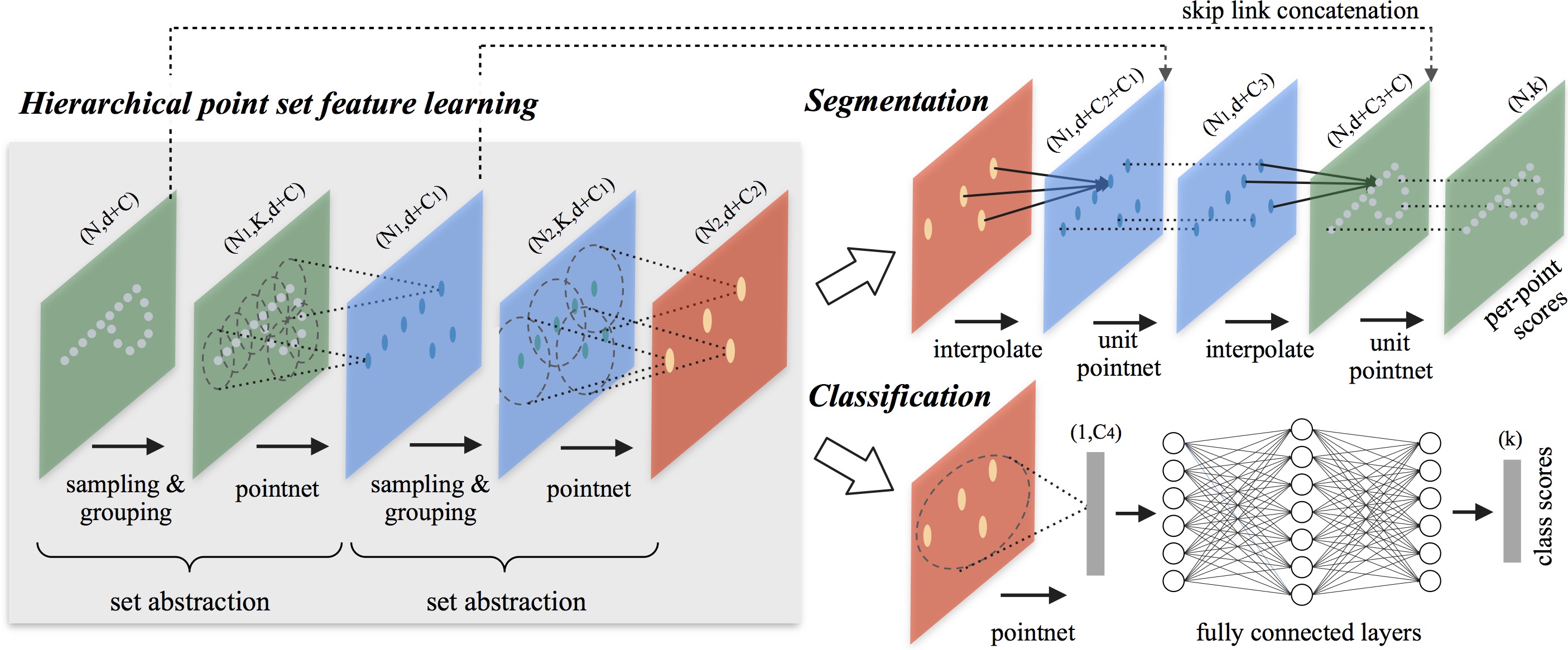 Figure 2. Diagram depicting PointNet++ architecture.
For our experiments we made use of the state-of-the-art Semantic3D and KITTI datasets. In Semantic3D, there is ground truth labels for 8 semantic classes: 1) man-made terrain, 2) natural terrain, 3) high vegetation, 4) low vegetation, 5) buildings, 6) remaining hardscape, 7) scanning artifacts, 8) cars and trucks. The goal for the point cloud classification task is to output per-point class labels given the point cloud.
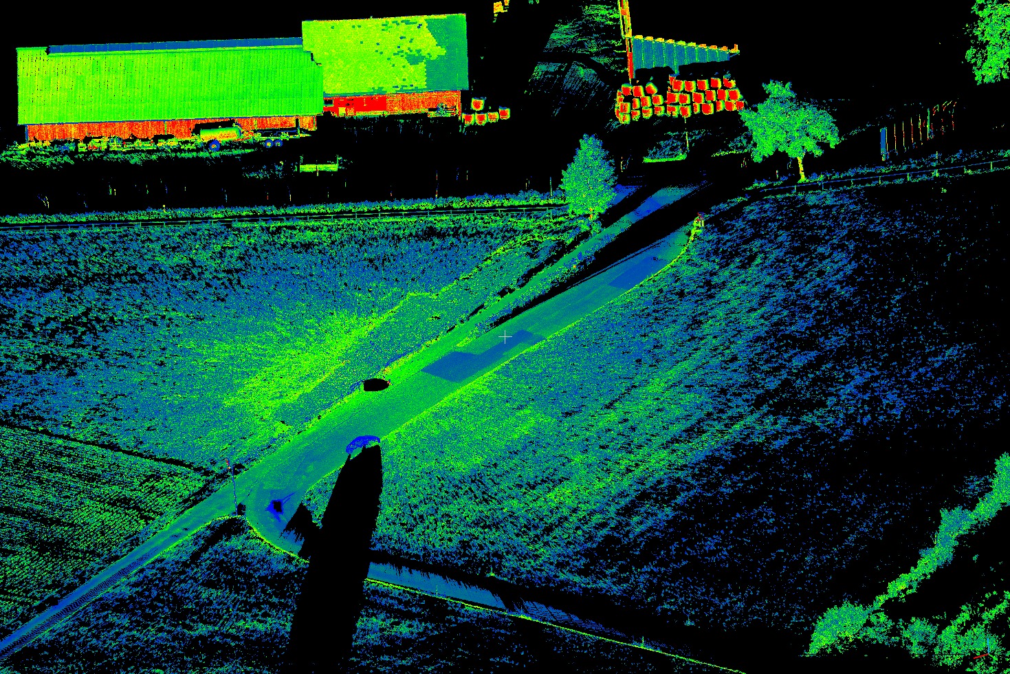 Figure 3. Semantic 3D snapshot
 Figure 4. KITTI snapshot
Since Semantic3D dataset contains a huge number of points per point cloud (up to 5e8, see dataset stats), we first run voxel-downsampling with Open3D to reduce the dataset size. During both training and inference, PointNet++ is fed with fix-sized cropped point clouds within boxes, we set the box size to be 60m x 20m x Inf, with the Z-axis allowing all values. During inference with KITTI, we set the region of interest to be 30m in front and behind the car, 10m to the left and right of the car center to fit the box size. This allows the PointNet++ model to only predict one sample per frame.
Our semantic segmentation model is trained on the Semantic3D dataset, and it is used to perform inference on both Semantic3D and KITTI datasets. In this document, we focus on the techniques which enable real-time inference on KITTI.
Accelerating PointNet++ with Open3D-enabled TensorFlow op
In PointNet++’s set abstraction layer, the original points are subsampled, and features of the subsampled points must be propagated to all of the original points by interpolation (see Section 3.4 of PointNet++). This is achieved by 3-nearest neighbors search, of which the authors provided a simple C++ implementation via custom TensorFlow op called ThreeNN. However, this turns out to be the bottleneck of the PointNet++ prediction model.
The following benchmark is obtained by the benchmark script running inference on a batch of 64 samples on colored Semantic3D dataset. As we can see, the ThreeNN op accounts for 87% of the graph execution time.
// Batch time
Batch size: 64, batch_time: 1.8208365440368652

// Per-op time
node name |           total execution time |  accelerator execution time |        cpu execution time |
ThreeNN            1.73sec (100.00%, 87.61%),        0us (100.00%, 0.00%),   1.73sec (100.00%, 95.87%)
ThreeInterpolate     60.68ms (12.39%, 3.07%),        0us (100.00%, 0.00%),      60.68ms (4.13%, 3.36%)
GroupPoint            27.31ms (9.32%, 1.38%),   27.03ms (100.00%, 15.85%),        275us (0.77%, 0.02%)
Conv2D                26.91ms (7.94%, 1.36%),    23.99ms (84.15%, 14.07%),       2.91ms (0.76%, 0.16%)
Open3D uses FLANN to build KDTrees for fast retrieval of nearest neighbors, which can be used to accelerate the ThreeNN op. This custom TensorFlow op implementation must be linked with Open3D and the TensorFlow library. To conveniently link the various dependencies, we provide a CMake file that automatically downloads, builds and links Open3D. When Open3D is properly installed (in this case automatically), one can simply use Open3D's CMake finder to include headers and link Open3D like the following.
target_include_directories(tf_interpolate PUBLIC ${Open3D_INCLUDE_DIRS})
target_link_libraries(tf_interpolate tensorflow_framework ${Open3D_LIBRARIES})
For more details on how to link a C++ project to Open3D, please see this documentation.
Next, we refactor the ThreeNN to make use of Open3D. In summary, first, a KDTree with the reference point is created by
open3d::KDTreeFlann reference_kd_tree(reference_pcd);Then for each target point, we search the 3 nearest neighbors in the KDTree
// for each j:
reference_kd_tree.SearchKNN(target_pcd.points_[j], 3, three_indices, three_dists);
After refactoring ThreeNN with Open3D, we see a ~2X speed up in both the ThreeNN and the full model run time with batch size 64.
// Batch time
Batch size: 64, batch_time: 0.7777869701385498

// Per-op time
node name |             total execution time |  accelerator execution time |         cpu execution time |
ThreeNN            694.14ms (100.00%, 73.72%),         0us (100.00%, 0.00%),   694.14ms (100.00%, 90.20%)
ThreeInterpolate      62.94ms (26.28%, 6.68%),         0us (100.00%, 0.00%),       62.94ms (9.80%, 8.18%)
GroupPoint            27.18ms (19.60%, 2.89%),    26.90ms (100.00%, 15.63%),         287us (1.62%, 0.04%)
Conv2D                26.39ms (16.71%, 2.80%),     23.83ms (84.37%, 13.85%),        2.56ms (1.58%, 0.33%)
Post processing: accelerating label interpolation
Since we subsampled the original dataset before feeding points to PointNet++, the network outputs only correspond to a sparse subset of the original point cloud.
 Figure 5. Inference on sparse pointcloud (KITTI).
 Figure 6. Inference results after interpolation.
The sparse labels need to be interpolated to generate labels for all input points. This interpolation can be achieved with nearest neighbor search using open3d.KDTreeFlann and majority voting, similar to what we did above in the ThreeNN op.
def interpolate_dense_labels(sparse_points, sparse_labels, dense_points, k=3):
    sparse_pcd = open3d.PointCloud()
    sparse_pcd.points = open3d.Vector3dVector(sparse_points)
    sparse_pcd_tree = open3d.KDTreeFlann(sparse_pcd)

    dense_labels = []
    for dense_point in dense_points:
        _, sparse_indexes, _ = sparse_pcd_tree.search_knn_vector_3d(
            dense_point, k
        )
        knn_sparse_labels = sparse_labels[sparse_indexes]
        dense_label = np.bincount(knn_sparse_labels).argmax()
        dense_labels.append(dense_label)
    return dense_labels
However, doing so in Python could be a major performance hit. We run the full kitti_predict.py inference on KITTI dataset for a benchmark. The interpolation step takes about 90% of the total run time and slows down the full pipeline to about 1 FPS.
$ python kitti_predict.py --ckpt path/to/checkpoint.ckpt
...
[ 1.05 FPS] load_data: 0.0028, predict: 0.0375, interpolate: 0.9076, visualize: 0.0031, total: 0.9545
[ 1.06 FPS] load_data: 0.0028, predict: 0.0355, interpolate: 0.8952, visualize: 0.0025, total: 0.9396
[ 1.04 FPS] load_data: 0.0028, predict: 0.0348, interpolate: 0.9214, visualize: 0.0024, total: 0.9653
...
To address the performance issue, another custom TensorFlow C++ op InterploateLabel is added. The op takes sparse_points, sparse_labels, dense_points and outputs dense_labels. OpenMP is used to parallelize KNN tree search. dense_colors output is also added to the op to directly output label-colored dense points. Please refer to the source code for details.
Another benefit of using such approach is that now the full pipeline of prediction and interpolation is implemented with one TensorFlow op graph. That is, TensorFlow session takes in the original dense points, and directly returns dense labels and label-colored dense points. This approach is more modular and efficient than doing the interpolation outside of the TensorFlow graph. After optimization, the end-to-end pipeline achieved an average of 10+ FPS on KITTI dataset, which faster than KITTI's capture rate at 10 FPS.
$ python kitti_predict.py --ckpt path/to/checkpoint.ckpt
...
[10.73 FPS] load_data: 0.0046, predict_interpolate: 0.0840, visualize: 0.0046, total: 0.0932
[12.89 FPS] load_data: 0.0047, predict_interpolate: 0.0693, visualize: 0.0035, total: 0.0776
[11.44 FPS] load_data: 0.0047, predict_interpolate: 0.0791, visualize: 0.0035, total: 0.0874
...
Video example on KITTI dataset
How-to train Open3D-PointNet++ on Semantic3D dataset
1. Data download
Download the Semantic3D dataset and extract
cd dataset/semantic_raw
bash download_semantic3d.sh
The outcome of these commands should look like this:
Open3D-PointNet2-Semantic3D/dataset/semantic_raw
├── bildstein_station1_xyz_intensity_rgb.labels
├── bildstein_station1_xyz_intensity_rgb.txt
├── bildstein_station3_xyz_intensity_rgb.labels
├── bildstein_station3_xyz_intensity_rgb.txt
├── ...
2. Convert txt to pcd file
Run
python preprocess.py
Open3D is able to read .pcd files much more efficiently.
Open3D-PointNet2-Semantic3D/dataset/semantic_raw
├── bildstein_station1_xyz_intensity_rgb.labels
├── bildstein_station1_xyz_intensity_rgb.pcd (new)
├── bildstein_station1_xyz_intensity_rgb.txt
├── bildstein_station3_xyz_intensity_rgb.labels
├── bildstein_station3_xyz_intensity_rgb.pcd (new)
├── bildstein_station3_xyz_intensity_rgb.txt
├── ...
3. Downsample
Run
python downsample.py
The downsampled dataset will be written to dataset/semantic_downsampled. Points with label 0 (unlabled) are excluded during downsampling.
Open3D-PointNet2-Semantic3D/dataset/semantic_downsampled
├── bildstein_station1_xyz_intensity_rgb.labels
├── bildstein_station1_xyz_intensity_rgb.pcd
├── bildstein_station3_xyz_intensity_rgb.labels
├── bildstein_station3_xyz_intensity_rgb.pcd
├── ...
4. Compile TF Ops
We need to build TF kernels in tf_ops. First, activate the virtualenv and make sure TF can be found with current python. The following line shall run without error.
python -c "import tensorflow as tf"
Then build TF ops. You'll need CUDA and CMake 3.8+.
cd tf_ops
mkdir build
cd build
cmake ..
make
After compilation the following .so files shall be in the build directory.
Open3D-PointNet2-Semantic3D/tf_ops/build
├── libtf_grouping.so
├── libtf_interpolate.so
├── libtf_sampling.so
├── ...
Verify that that the TF kernels are working by running
cd .. # Now we're at Open3D-PointNet2-Semantic3D/tf_ops
python test_tf_ops.py
5. Train
Run
python train.py
By default, the training set will be used for training and the validation set will be used for validation. To train with both training and validation set, use the --train_set=train_full flag. Checkpoints will be output to log/semantic.
6. Predict
Pick a checkpoint and run the predict.py script. The prediction dataset is configured by --set. Since PointNet2 only takes a few thousand points per forward pass, we need to sample from the prediction dataset multiple times to get a good coverage of the points. Each sample contains the few thousand points required by PointNet2. To specify the number of such samples per scene, use the --num_samples flag.
python predict.py --ckpt log/semantic/best_model_epoch_040.ckpt \
                  --set=validation \
                  --num_samples=500
The prediction results will be written to result/sparse.
Open3D-PointNet2-Semantic3D/result/sparse
├── sg27_station4_intensity_rgb.labels
├── sg27_station4_intensity_rgb.pcd
├── sg27_station5_intensity_rgb.labels
├── sg27_station5_intensity_rgb.pcd
├── ...
7. Interpolate
The last step is to interpolate the sparse prediction to the full point cloud. We use Open3D's K-NN hybrid search with specified radius.
python interpolate.py
The prediction results will be written to result/dense.
Open3D-PointNet2-Semantic3D/result/dense
├── sg27_station4_intensity_rgb.labels
├── sg27_station5_intensity_rgb.labels
├── ...
8. Submission
Finally, if you're submitting to Semantic3D benchmark, we've included a handy tools to rename the submission file names.
python renamer.py
9. Summary of directories
dataset/semantic_raw: Raw Semantic3D data, .txt and .labels files. Also contains the .pcd file generated bypreprocess.py.dataset/semantic_downsampled: Generated fromdownsample.py. Downsampled data, contains .pcd and .labels files.result/sparse: Generated frompredict.py. Sparse predictions, contains .pcd and .labels files.result/dense: Dense predictions, contains .labels files.result/dense_label_colorized: Dense predictions with points colored by label type.
How-to train and validate Open3D-PointNet++ on the KITTI dataset
This section provides additional information on how to train a model to work with the KITTI dataset
1. Data download and preparation
2. Install auxiliary dependencies
pip install pykitti3. Training with adapted Semantic3D data
3. Perform real-time Inference